Cobra Survival

Introduction

from cobsurv.models import CobraSurvival
import pandas as pd
from sklearn.model_selection import train_test_split
from sksurv.datasets import load_flchain

Lets load Dataset flchain

X , y = load_flchain()

Let’s Preprocess the dataset

X_dummy = pd.get_dummies(X)
# remove rows with missing values
index_missing = X_dummy.isna().any(axis=1)
X_dummy = X_dummy.loc[~index_missing]
y = y[~index_missing]

Let’s split the dataset into train and test

X_train, X_test, y_train, y_test = train_test_split(X_dummy.values, y, test_size=0.01 , random_state = 20 , shuffle = True)

Lets fit the model, with \(\epsilon = 0.3\) and \(\alpha = 4\) and using trapz as distance function, there are other distance function available, like euler , euclidean, shannon-jensen etc.

cbr = CobraSurvival(epsilon = 0.11, alpha = 3, distance_function='trapz')
cbr.fit(X_train,y_train)

CobraSurvival(alpha=3, distance_function='trapz', epsilon=0.11)

In a Jupyter environment, please rerun this cell to show the HTML representation or trust the notebook.
On GitHub, the HTML representation is unable to render, please try loading this page with nbviewer.org.

We may get sometime, the number of quantile warning, is due to the fact that the \(D_k\) and \(D_l\) split is done by time quantile and censoring, this happening that every quantile is not getting same proportion, so that it is reducing the number of quantile to get the same proportion.

Predict

The prediction from a cobra survival model is the probability of survival at a attribute unique_sorted_times_l also with default machine option we can get scikit-survival base estimators.

cbr.predict(X_test)

array([[1.        , 1.        , 1.        , ..., 0.99037084, 0.99037084,
        0.99037084],
       [1.        , 1.        , 1.        , ..., 0.99051196, 0.99051196,
        0.99051196],
       [0.99688474, 0.99688474, 0.99376947, ..., 0.        , 0.        ,
        0.        ],
       ...,
       [1.        , 1.        , 1.        , ..., 0.97820437, 0.97820437,
        0.97820437],
       [1.        , 1.        , 1.        , ..., 0.99212188, 0.99212188,
        0.99212188],
       [1.        , 1.        , 1.        , ..., 0.99036519, 0.99036519,
        0.99036519]])

Plotting

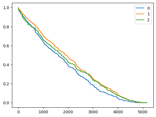
We can plot the survival curve using, plot method, which take the covariates and the index of the observation whose plot is needed, the plot is supported by pycox.evaluation, so only fifty index is supported, suppose we want to plot 4,5 and 8

import matplotlib.pyplot as plt
%matplotlib inline

index = [4,5,8] # these are the observations for which we want to plot the survival curve
X_to_plot = X_test[index]
cbr.plot(X_to_plot , [0,1,2])
plt.show()

Score

The Integrated Brier Score can be calculated using score method, when type is concordance it will return the concordance index, when type is ibs it will return the integrated brier score.(defualt is ibs)

cbr.score(X_test, y_test)

0.03228505500485323

cbr.score(X_test,y_test, type = 'concordance')

0.956359102244389